We’ve hosted a webinar aimed specifically at non-ferrous melt analysis and our OES expert Jochen Meurs covered 5 key areas of non-ferrous OES. If you missed it, you can watch the recording here.
We gave those attending the opportunity to submit questions and these were excellent and required in-depth answers. In this article we’ve collected all the questions that related to understanding measurements and detection limits in OES. These are the answers given by Jochen Meurs.
In the presentation we discussed results for milled samples vs ground samples to demonstrate the difference in precision for the two sample preparation methods.
Question: Why is the result for titanium (Ti) so much higher in the ground sample than the milled sample?
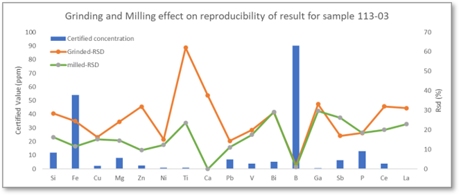
The graph is a visual presentation of the reproducibility of the results for the two preparation methods (not the absolute value for composition) and therefore plots the relative standard deviation (RSD) for measurements taken with each type of sample. RSD is the standard deviation expressed as a percentage of the average concentration value and is therefore related to precision. For the ground samples, the measurements fluctuate between 2 - 11 ppm, whereas for the milled samples, we get much better precision with a fluctuation between 1 - 3 ppm.
Bearing in mind that the limit of detection for Ti is 1ppm, we see the maximum precision that’s statistically possible with the milled sample. The reason why ground samples show much less precision is not clear. It could be that particles transferred from the grinding disc influence the results, especially as Ti can be present in substances used to produce the disc. Another reason (according to studies by Thyssen Krupp steel works) is that the roughness is not uniform after grinding, due to the paper grain, or fluctuations in the force applied to the sample.
Whatever the root cause of lack of precision when grinding, milling is certainly more reproducible when investigating surface roughness and possible contamination, especially when using an automated mill where parameters are exactly the same each time you prepare a sample.
We explained why such a large range of elements need to be analyzed for non-ferrous materials, and why a high-performance CMOS-based OES spectrometer is the best solution.
Question: Are there any limitations on measuring elements for Al alloy analysis with CMOS detectors? What about rare earth elements, such as Sc (scandium)?
We cover scandium as part of our in-house calibration for aluminum alloys for the OE750 (for concentrations between 0.00005 – 0.06%). Other rare earth elements are theoretically feasible, but the problem is that there are no certified standards available on the market for instrument calibration. This is the only limiting factor for measuring rare earths in aluminum with the CMOS detector as suitable emission lines are available.
If you take a look at our Mg and Al-calibration application notes, you can see what’s possible.
Question: How can one obtain more accurate N and C analysis at low levels?
Both elements are very sensitive to sample preparation. They must be ground or milled immediately prior to analysis. The challenge for nitrogen is that it’s present in the air. It only takes a few hours before N from the atmosphere will adhere to the sample surface – this will give you an artificially high reading for N. This also means that you need a perfect seal between the spark stand and sample (again, any air entering this space will give a high reading for nitrogen). With carbon, the issue is dirt and contamination on the surface. The surface must be clean and freshly prepared.
I strongly recommend argon 6.0 or a suitable purifier. Only this type of gas will allow for the reliable detection of nitrogen at a level below 100 ppm. For our highest performing OES instruments (OE750 and FOUNDRY-MASTER Pro2), we insist on Ar 6.0 when analyzing gases.
Question: When the concentration percentage is on the X-axis and the intensity on the Y-axis, why is the line linear at very low concentrations (<100 ppm) but then levels off as the concentration increases?
This is called the reversal effect, and some emission lines are more sensitive to this than others. This is due to self-absorption of the emitted light. At low concentrations there is negligible self-absorption; all the emitted light reaches the detector and the curve is linear. However, as the concentration (and density) of a particular element increases, more of the emitted light will be re-absorbed by the plasma before it has a chance to reach the detector. This is where we lose our linear relationship and the curve levels off.
A well-known effect of this is the Cu 327.4 nm line in steel. The reversal means the use of this line is effective only for Cu concentrations less than 1%. Above this level, you must select a less sensitive line, such as Cu 510 nm. This is the reason why OES spark spectrometers use different emission lines for one element, depending on the concentration range. In glow-discharge OES, you always have a low-density plasma due to the low pressure in the discharge chamber, and here you get linear calibration curves.
Question: You have mercury listed as an analyzed element for aluminum. I thought that OES was not a recommended method for Hg.
This is correct, but OES is often used to monitor unwanted or harmful elements. In general, spectroscopy is a very sensitive method and detects the presence of elements very well. However, the accurate measurement of an element at a given concentration is challenging if there are no suitable reference materials available.
This is our calibration of Hg on the OE750:
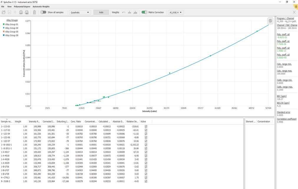
The detection limit for Hg is between 5 - 10 ppm, and this calibration should allow for monitoring and give a semi-quantitative result. This is similar to C and S determination in steel; the reference method is combustion analysis, but for monitoring the steel-making process, spark-OES results give the information required, and is much faster than combustion analysis.
If you’d like to see the recording of the live webinar Best 5 expert tips for optimal non-ferrous melt control with spark OES, you can watch it here.
In our new guide Optimal non-ferrous melt control with spark OES, we go into more detail on the optimum sample-taking process and preparation techniques to get reliable results first time when verifying non-ferrous melt chemistry. Download your copy by clicking on the link above or on the button below.
Get the guide Watch the webinar recording