The internationally approved method for calculating measurement uncertainty – GUM – relies on the availability of a certified reference sample. Similarly, reference samples are also used to find any repeatable offset (systematic deviation of the mean) of your analyser.
But what do you do when you don’t have a reference sample to hand? Or the one you have is not within the region of interest for your current measurement? You can get round this by applying different statistical methods. But before we go into the methods, we need to look at what we mean by measurement uncertainty.
As we’ve discussed in a previous post on measurement errors, an accurate reading needs to fulfil two criteria:
Accuracy of the mean (trueness). This is how far the mean of our measurements deviates from the expected result. Measurement errors due to this show as a systematic deviation of the mean for every measurement we make in our instrument.
Precision. If we take the same measurement several times, precision is a measure of how similar the results are. Poor precision shows a large fluctuation each time, whereas good precision gives results that are close together. Precision is due to random fluctuations, so the results follow a normal distribution.
We’ll need to calculate both of these and then combine the result to get an overall confidence interval for accuracy.
If we had a reference sample of known composition, we’d simply compare the certified value to our own averaged measured values and apply the resulting offset to all our results. When that option isn’t available, we have to use another method – the Standard Error of the Estimate or SEE.
The equation for the standard error of the estimate is given below:
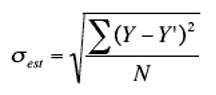
Where:
σest is the standard error of the estimate
Y is the actual result measured by the instrument
Y’ is the result after regression analysis
N is the number of values
It’s easier to see how this works, if we use some real numbers. Here’s a table of results from a spectrometer.
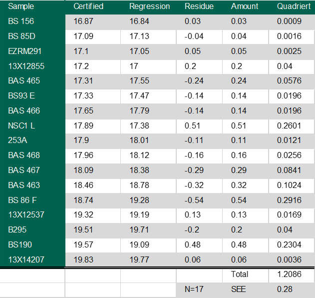
The first column of figures are the measured values, the second is the result after the software has applied the regression analysis. Using these numbers in the above formula gives us a standard error of the estimate of 0.28%.
When we can’t use the GUM method for measurement uncertainty due to random fluctuations, we rely on the Student t-distribution function. This distribution function was developed when the number of samples is very low.
The confidence interval given by the Student t-distribution function is given by:
uc= X̅+/- TX̅
Where:
X̅: average of the measured values
TX: value of the t-distribution function. This is calculated from the following formula:
Tx= (t (f,P) x s / N1/2
Where:
t: value taken from published tables which depends on f (number of samples measured - 1) and P (the desired confidence level).
s: standard deviation of the measurement series
N: number of measurements taken
Let’s assume we’ve measured an unknown sample 10 times and have the following results for chromium composition:
Average composition from 10 readings: 18.82%
Standard deviation 0.15%
We’ll work within a confidence level of 95%, which means that the values we need to plug into the above formulae are:
n: 10
P: 95%
s: 0.15%
t: 2.262 (for P of 95% and sample size 10)
Working through these numbers gives us a confidence level
Uc = +/-0·11%
Now we’ve got everything we need to calculate the overall measurement uncertainty. All we do is add our value of +/- 0.11% for precision to the value of +/-0.28 for accuracy of the mean and we get our final result:
C = 18.82 % +/- 0.39% @ 95% probability.
We cover this method in detail in our Search for True Values guide, including how to evaluate accuracy and calculate the error margin of spectroscopy measurements. This guide begins by covering basic statistics and then walks you through different methods of calculating measurement uncertainty for your own spectroscopy measurements. Download your copy here.